Polar Coordinates
Mathematicians translate between geometry and algebra using “coordinates”, assignments of ordered lists of numbers to geometric locations. To define rectangular coordinates in the plane, see our blog post on functions, coordinates, and graphs, we fix perpendicular “axes”: a horizontal and a vertical number line meeting at a point called the “origin”, let \(x\) denote position along the horizontal axis and \(y\) denote position along the vertical axis, and thereby associate to each ordered pair \((x, y)\) of real numbers a unique point of the plane. Conversely, each point of the plane has unique rectangular coordinates once the axes are fixed.
“Polar coordinates” are an alternative system of coordinates in the plane. Define the polar ray to be the positive horizontal axis. Polar coordinates are the distance \(r\) to the origin, and the angle \(\theta\) measured counterclockwise from the polar ray, see our blog post on circles, trigonometry, and groups.
A rectangular grid is a collection of lines where \(x\) is constant or \(y\) is constant, with several evenly-spaced values for each coordinate. Similarly, a polar grid is a collection of curves where \(r\) is constant or \(\theta\) is constant.
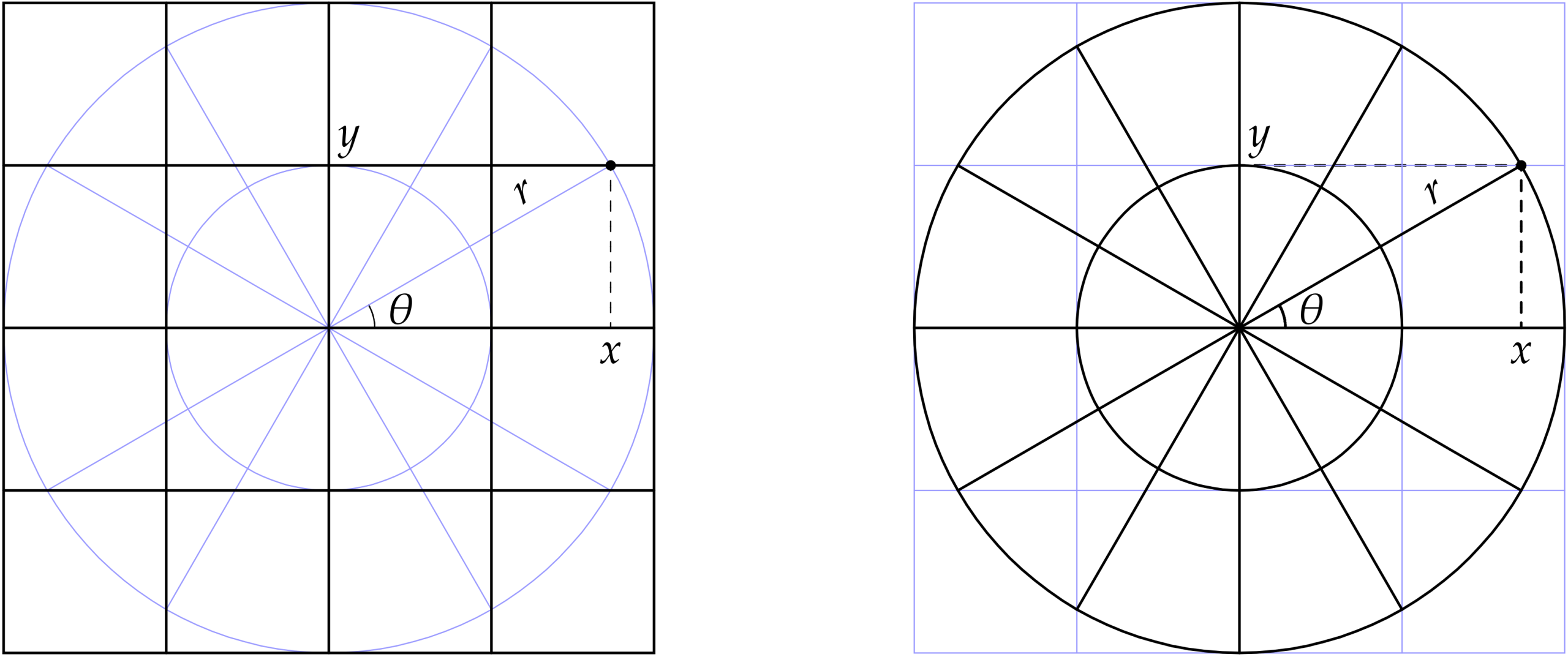
Overlaying two types of grid emphasizes that each is extra structure giving an algebraic description of the same underlying geometric reality.
Given a distance and heading \((r, \theta)\), there is a unique point in the plane with that distance and heading. Its rectangular coordinates are given by
\[
(x, y) = (r\cos\theta, r\sin\theta).
\]
These formulas make sense if \(r\) is not positive, so we usually do not restrict \(r\) or \(\theta\).
Unlike with rectangular coordinates, each point in the plane has infinitely many sets of polar coordinates. For example, \(P(1, 0) = (1, 0) = P(1, 2\pi)\). Generally, if \(r\) is non-zero, then for every integer \(k\) we have
\begin{align*}
P(r, \theta + 2\pi k) &= P(r, \theta), \\
P(-r, \theta + \pi + 2\pi k) &= P(r, \theta).
\end{align*}
Inversely, these are the only situations with \(r \neq 0\) where distinct polar coordinates give the same rectangular location. (If \(r = 0\), the angle is immaterial: \(P(0, \theta) = (0, 0)\) for all real \(\theta\). We do not speak of the origin as having a polar angle.)
Polar Graphs
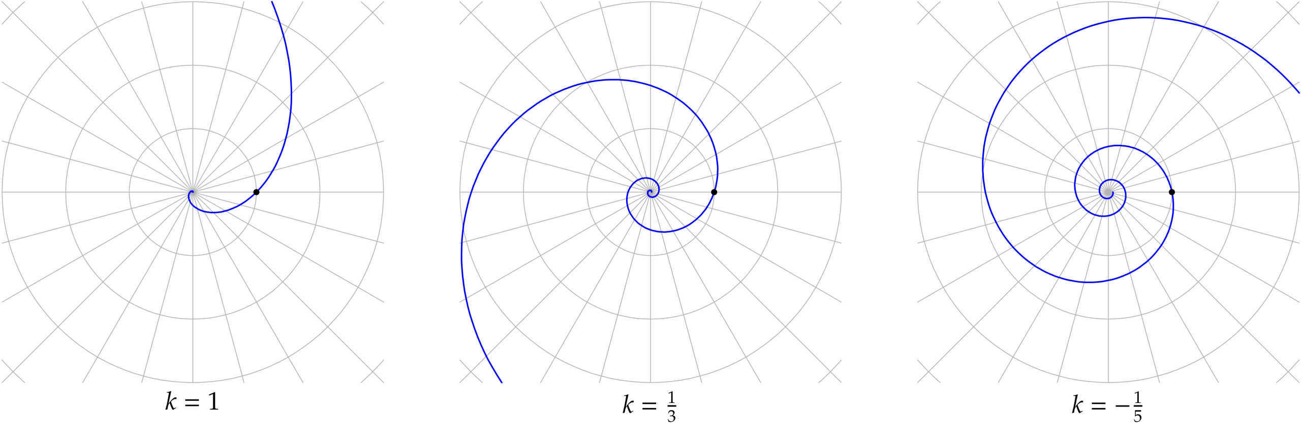
An equation such as \(r = e^{\theta}\) defines a polar graph. For each real \(\theta\) we calculate the radius \(r = e^{\theta}\) and plot the point with polar coordinates \((r, \theta)\). This particular polar graph, a “logarithmic spiral,” is a favorite at Differential Geometry. It, and closely-related curves, may be found in our series Flow Sphere, Loxodromes, and Tendrils.
More generally, if \(k\) is a non-zero real number, the polar graph \(r = e^{k\theta}\) is called a logarithmic spiral. Mathematically, a logarithmic spiral is the path traced out as the plane “rotates-and-scales at constant angular speed.” The parameter \(k\) corresponds to the direction of winding and tightness of the spiral. If \(k\) is positive, the spiral winds outward as we proceed counterclockwise, and if \(k\) is negative the spiral winds inward. The closer \(|k|\) is to \(0\), the less \(e^{k\theta}\) grows or shrinks when \(\theta\) advances by \(2\pi\), i.e., as the graph makes one full turn about the origin, and the tighter the spirals winds.
Even if you have not heard of logarithmic spirals, these curves may be a favorite of yours, too: Cross sections of sea shells are well-approximated by logarithmic spirals! Biologically, a mollusk grows, to a good approximation, by expanding in size due to accretion onto an existing structure. The result is rotation-and-scaling at constant angular speed.
Regardless of \(k\), the logarithmic spiral \(r = e^{k\theta}\) passes through the rectangular point \((1, 0)\), because \(e^{0} = 1\). If we follow the spiral counterclockwise, we increase the polar angle \(\theta\). Making one full turn corresponds to incrementing \(\theta\) by \(2\pi\). By the law of exponents,
\[
e^{k(\theta + 2\pi)} = e^{k\theta + k(2\pi)}
= e^{k\theta} \cdot \underbrace{e^{k(2\pi)}}_{\text{scale factor}}.
\]
Geometrically, rotating the logarithmic spiral \(r = e^{k\theta}\) one turn counterclockwise has the same effect as scaling the spiral by a factor \(e^{k(2\pi)} = e^{2\pi k}\). This is a quantitative expression of our qualitative rotate-and-scale description.
Geometrically, there is no difference between rotating a logarithmic spiral about the origin and scaling the spiral uniformly about the origin! Is this spiral rotating counterclockwise, or uniformly shrinking? Yes.
Polar coordinates tend to simplify descriptions of plane curves and shapes having rotational symmetry about the origin. Every real-valued function \(f\) has a rectangular graph \(y = f(x)\), comprising all rectangular points \((x, y)\) with \(y = f(x)\). Analogously, the polar graph \(r = f(\theta)\) comprises all polar points \((r, \theta)\) with \(r = f(\theta)\).
The rose curves \(r = a\cos(k\theta)\), with \(a\) and \(k\) positive real numbers, have pleasing symmetry, particularly when \(k\) is a fraction with small denominator. Curves related to roses may be found in our Dipole Sphere series.
One remarkable example is the polar graph \(r = \cos\theta\), often seen when students learn to convert between rectangular and polar coordinates. If we multiply the defining equation by \(r\), we obtain the equivalent polar equation \(r^{2} = r\cos\theta\). Let \((x, y)\) denote rectangular coordinates. By the hypotenuse theorem, \(r^{2} = x^{2} + y^{2}\). Further, as we saw earlier, \(x = r\cos\theta\). Substituting, we conclude that
\[
x^{2} + y^{2} = r^{2} = r\cos\theta = x,
\]
or \(x^{2} – x = 0\). As we’ll see next, this is the equation of a circle passing through the origin.
In our blog post on circles, trigonometry, and groups, we saw that the circle of center \((x_{0}, y_{0})\) and radius \(r\) has rectangular equation
\[
(x – x_{0})^{2} + (y – y_{0})^{2} = r^{2}.
\]
We will show that \(x^{2} – x = 0\) can be re-written
\[
\bigl(x – \tfrac{1}{2}\bigr)^{2} = \bigl(\tfrac{1}{2}\bigr)^{2},
\]
the equation of the circle with center \((x_{0}, y_{0}) = (\frac{1}{2}, 0)\) and radius \(r = \frac{1}{2}\).
There is a systematic algebra procedure, “completing the square,” that here may be viewed as writing
\begin{align*}
x^{2} – x &= x(x – 1) && \text{factoring} \\
&= \bigl(x – \tfrac{1}{2} + \tfrac{1}{2}\bigr)
\bigl(x – \tfrac{1}{2} – \tfrac{1}{2}\bigr)
&& \text{sneaky!} \\
&= \bigl(x – \tfrac{1}{2}\bigr)^{2} – \bigl(\tfrac{1}{2}\bigr)^{2}
&& \text{difference of squares.}
\end{align*}
Consequently, the equation \(x^{2} – x = 0\) may be written \(\bigl(x – \tfrac{1}{2}\bigr)^{2} – \bigl(\tfrac{1}{2}\bigr)^{2} = 0\). Adding \(\bigl(\tfrac{1}{2}\bigr)^{2}\) to both sides and canceling terms on the left gives
\[
\bigl(x – \tfrac{1}{2}\bigr)^{2} = \bigl(\tfrac{1}{2}\bigr)^{2}.
\]
This particular polar graph is deceptively simple. The animation loop, worth a thousand words, shows a line through the origin rotating at constant angular speed, and the corresponding point on the polar graph \(r = \cos\theta\) (blue). Particularly, points on the polar graph correspond to lines through the origin, or to diametrically opposite pairs of points on the unit circle (black):
The topic of polar coordinates was part of the American pre-calculus curriculum of the 1970s, but has since largely been omitted. There is considerable appeal to curves that can be described by polar graphs. I hope this introduction to logarithmic spirals and rose curves has whetted your mathematical appetite, and encourages you to seek out more extensive catalogs of curves!