\(\DeclareMathOperator{\im}{Im}\DeclareMathOperator{\re}{Re}\DeclareMathOperator{\Arg}{Arg}\DeclareMathOperator{\pow}{\mathtt{pow}}\DeclareMathOperator{\Sqrt}{\mathtt{sqrt}}\)In this post we’ll build a bridge starting with the parabola familiar from plane geometry and arriving at the “Riemann surface of the complex square root,” which often mystifies complex analysis students. We’ll refer to complex numbers, coordinate geometry, and mappings. We’ll also draw pictures guided by coordinate geometry in more than three dimensions. Concretely, we’ll write lists of numbers with more than three entries, and treat these entries as spatial coordinates even though we cannot draw four mutually-perpendicular coordinate axes.
The Real Square Root
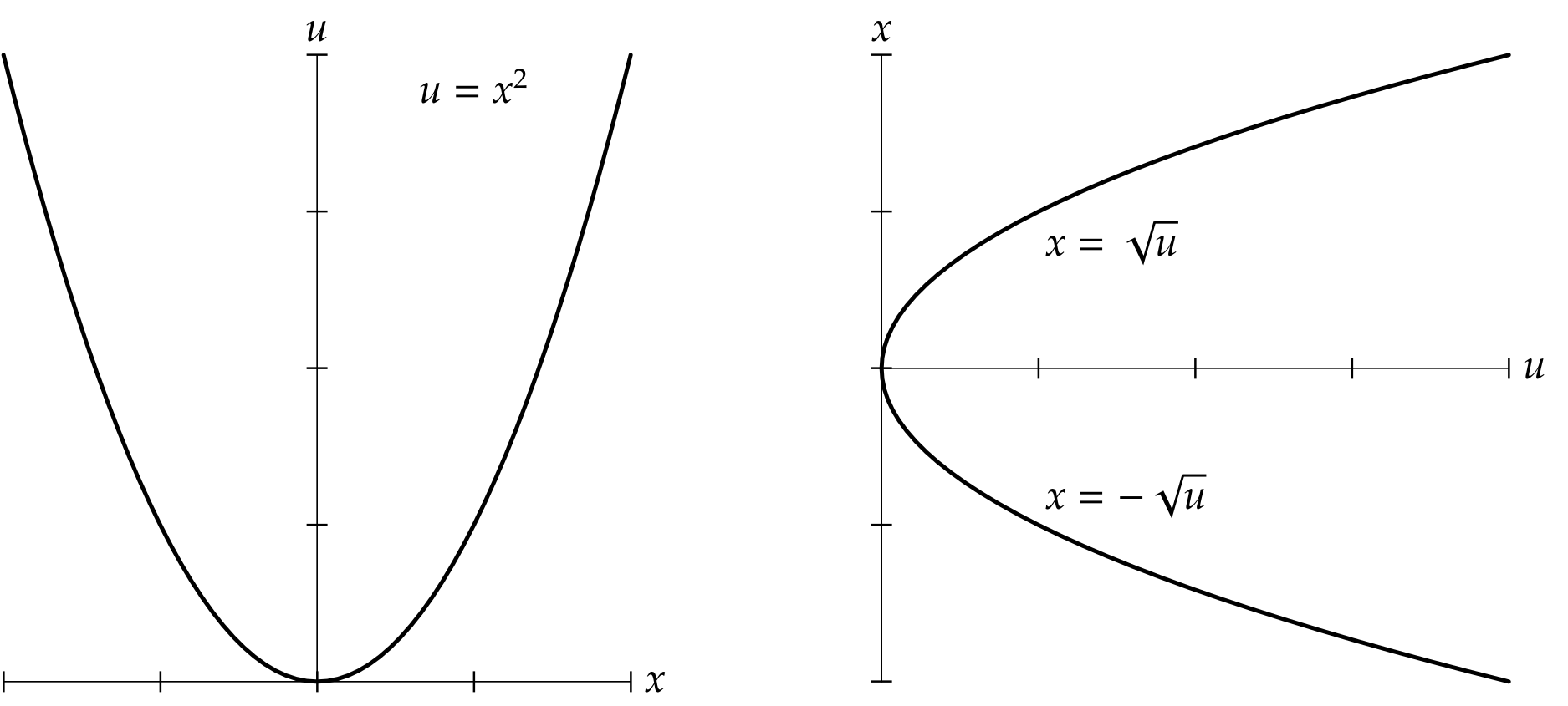
The Cartesian equation \(y = x^{2}\) defines a parabola, the graph of the real squaring function \(f(x) = x^{2}\). If we exchange the roles of the variables and solve for \(x\) as a function of \(y\), we obtain precisely two continuous choices of inverse: \(x = \sqrt{y}\) and \(x = -\sqrt{y}\), each defined where \(y \geq 0\).
For consistency of notation when we “complexify” it’s convenient to replace the Cartesian coordinate \(y\) with the less-conventional letter \(u\) now. Our parabola then has equation \(u = x^{2}\), and the two branches of inverse have equations \(x = \sqrt{u}\) and \(x = -\sqrt{u}\), each defined where \(u \geq 0\).
Our goal is to extend this picture to the complex plane. Surprisingly, we encounter a literal twist: If we let \(u\) trace a closed path around the origin of the complex plane, \(\sqrt{u}\) and \(-\sqrt{u}\) do not remain separate, but instead continuously change places.
The Complex Square Root
To complexify our equation \(u = x^{2}\), we’ll replace the real variable \(u\) with the complex variable \(w = u + iv\). When \(v = 0\) we have \(w = u\); in other words, \(u\) is the real part of \(w\), and \(w\) extends \(u\) to the complex plane.
Similarly, we’ll replace the real variable \(x\) with the complex variable \(z = x + iy\), which extends \(x\) to the complex plane. Our goal is to study the equation \(w = z^{2}\), with the hope of expressing \(z\) as a function of \(w\).
It turns out every non-zero complex number \(w\) has a non-zero complex square root. We’ll be able to justify this presently. To give a couple of examples for now, \(i\) is a square root of \(-1\), and \((1 + i)/\sqrt{2}\) is a square root of \(i\). You may wish to check these for yourself as practice with
multiplying complex numbers.
We can check that every complex number \(w\) has at most two complex square roots: If \(w = s^{2}\) and \(w = t^{2}\), then
\begin{align*}
0 &= t^{2} – s^{2} \\
&= (t – s)(t + s),
\end{align*}
so either \(t = s\) or \(t = -s\). We might therefore hope to define two branches of square root where \(w \neq 0\). To see if this is feasible, let’s try to draw the “complex parabola” \(w = z^{2}\).
Recall that we are writing \(w = u + iv\) and \(z = x + iy\), and are considering the equation \(w = z^{2}\). Multiplying out the right-hand side, we find
\begin{align*}
z^{2} &= (x + iy)(x + iy) \\
&= (x^{2} – y^{2}) + i(2xy).
\end{align*}
If \(w = u + iv = z^{2}\), then by equating real and imaginary parts we have \(u = x^{2} – y^{2}\) and \(v = 2xy\). In other words, the graph \(w = z^{2}\) is the set of points of the form
\begin{align*}
(z, w)
&= (z, z^{2}) \\
&= (x + iy, x^{2} – y^{2} + 2xyi).
\end{align*}
with \(x\) and \(y\) real.
If we identify \(z = x + iy\) with the real ordered pair \((x, y)\) and \(w = u + iv\) with \((u, v)\), we may identify the complex ordered pair \((z, w)\) with the real quadruple \((x, y, u, v)\). The calculation above expresses the graph \(w = z^{2}\) as the parametric surface
\[
(x, y, x^{2} – y^{2}, 2xy)
\]
with \(x\) and \(y\) real.
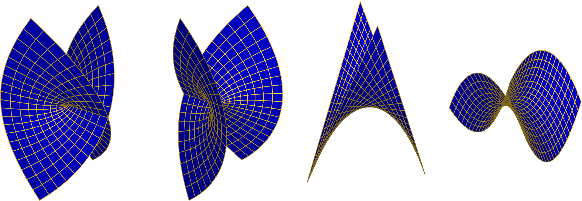
We cannot plot this surface directly because it sits in four-space. We can, however, project to three-space by discarding one coordinate, obtaining a surface we can plot. Discarding coordinates \(x\), \(y\), \(u\), and \(v\) in succession, we obtain four “shadows” of our complex parabola. The respective coordinates are \((y, u, v)\), \((x, u, v)\), \((x, y, v)\) and \((x, y, u)\).
If we work in polar coordinates \(x = r\cos\theta\) and \(y = r\sin\theta\), the polar formula
\[
e^{i\theta} = \cos\theta + i\sin\theta
\]
allows us to write
\begin{alignat*}{2}
z &= x + iy &&= re^{i\theta}, \\
w &= u + iv &&= r^{2} e^{2i\theta}.
\end{alignat*}
Our complex parabola is now parametrized by
\begin{align*}
(z, z^{2})
&= \bigl(re^{i\theta}, r^{2}e^{2i\theta}) \\
&= \bigl(r\cos\theta, r\sin\theta, r^{2}\cos(2\theta), r^{2}\sin(2\theta)\bigr).
\end{align*}
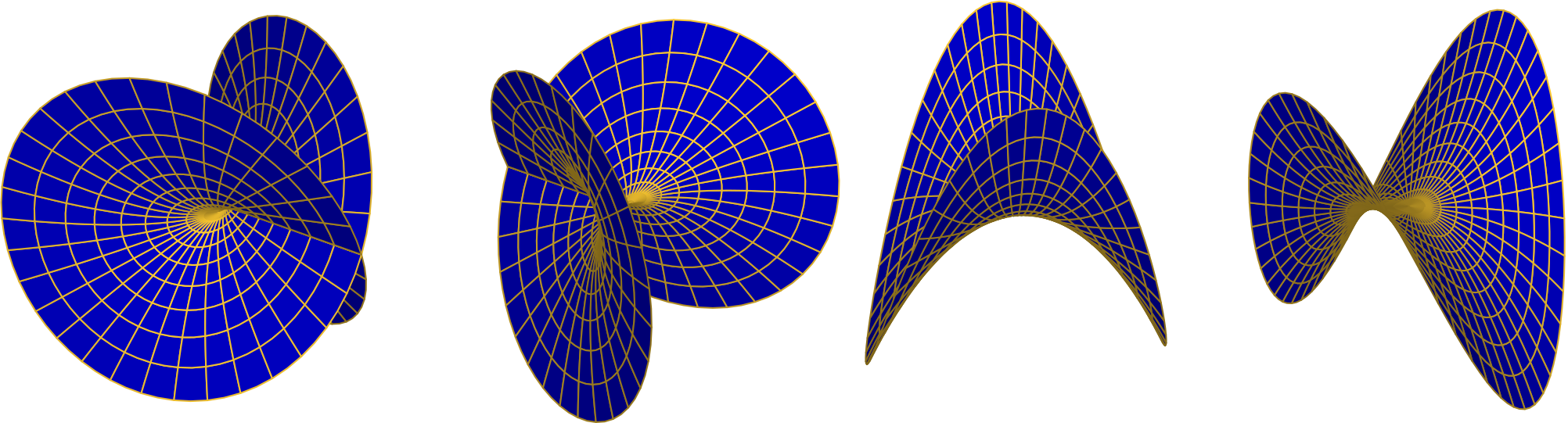
The qualitative similarity between these polar graphs and the earlier rectangular graphs should be visually apparent.
Inspection of these surfaces, especially the first and second, already suggests the trouble we’ll encounter trying to define branches of square root. In the first two pictures, the \(w\)-plane is fully shown, and contains a line of self-intersection and the vertical axis of the screen. The squaring map wraps a disk about the origin onto the surface, then projects orthogonally to the \(w\)-plane. The square root should “undo” this.
The problems are, there are two “sheets” over the \(w\)-plane corresponding to the two choices of square root of \(w\), and these sheets smoothly cross-join each other as we walk around the origin in the \(w\)-plane. To explore and understand these qualitative claims in detail, it helps to calculate using polar coordinates.
In polar coordinates, we wish to solve for \(z = re^{i\theta}\) in terms of \(w = r^{2} e^{2i\theta} = \rho e^{i\phi}\). The magnitudes pose no problem: \(|z| = r = \sqrt{\rho} = \sqrt{|w|}\). Because \(\rho\) and \(r\) are non-negative, we have only the non-negative real square root.
The polar angles might also appear straightforward. Formally, \(\theta = \frac{1}{2}\phi\). The snag is that each non-zero complex number \(w = \rho e^{i\phi}\) has infinitely many choices of polar angle \(\phi + 2\pi ki\) for some integer \(k\). This gives infinitely many choices for the polar angle of \(z\), namely \(\theta = \frac{1}{2}\phi + \pi ki\). But the choice of \(k\), while immaterial for \(w\), is consequential for \(z\) because
\begin{align*}
e^{k\pi i}
&= \cos(k\pi) + i\sin(k\pi) \\
&= \cos(k\pi) \\
&= \begin{cases}
\phantom{-}1 & \text{\(k\) even,} \\
-1 & \text{\(k\) odd.}
\end{cases}
\end{align*}
Let’s look more closely at what this equation tells us about square roots.
First, polar coordinates confirm a claim made earlier: Every non-zero complex number \(w\) has two square roots. Polar coordinates independently confirm that these square root differ by a sign.
Second, polar coordinates show that walking around the origin in the \(w\)-plane, which advances the polar angle \(\phi\) by \(2\pi\), advances the polar and \(\theta\) of \(z\) by only \(\pi\). When we complete one full circuit in \(w\), the square root has changed sign rather than returning to its starting value.
Further, a second traversal of the origin, incrementing \(\phi\) by \(2(2\pi) = 4\pi\), increments \(\theta\) by \(2\pi\) and returns the square root to its starting value. To emphasize, the square root “function” \(z = \sqrt{w}\) changes sign each time we walk once around \(w = 0\). We must circle the origin twice before the square root returns to its original value. Ordinary functions do not behave this way!
The Principal Square Root
In order to define a single-valued square root function on the \(w\)-plane, we must commit to a specific choice of polar angle for \(w\). By definition, the “principal” choice satisfies \(-\pi < \phi \leq \pi\). This choice is single-valued, and defines the principal square root \(z = \sqrt{w}\). The polar angle \(\theta\) of the principal square root satisfies \(-\frac{1}{2}\pi < \theta \leq \frac{1}{2}\pi\). That is, the point \(z = \sqrt{w}\) lies in the right half-plane \(0 \leq \re z\).
One vexing issue is the discontinuity of the principal angle, which jumps between \(-\pi\) and \(\pi\) across the negative real axis. On the negative real axis the polar angle \(\theta\) therefore jumps between \(-\frac{1}{2}\pi\) and \(\frac{1}{2}\pi\). Thus, for example, \(\sqrt{-1} = i\), but \(\sqrt{-1 – 10^{-40}i} \approx -i\). We'll see ways to visualize this below.
To emphasize, on the negative real axis, \(\sqrt{w} = \sqrt{|w|} i\) has positive imaginary part, but just below the negative real axis \(\sqrt{w} \approx -\sqrt{|w|} i\) has negative imaginary part. The principal square root is not continuous on the negative real axis.
Another annoyance affects algebra. After learning to rely on the identity \(\sqrt{rs} = \sqrt{r} \sqrt{s}\), new visitors to the complex plane are often surprised to find that this property does not hold: The product on the right might lie in the left half-plane, where \(\re z < 0\), while the left-hand side does not. We can only guarantee that if the product on the right lies in the right half-plane, the formula does hold.
The graphs of the real and imaginary parts of the principal square root, as functions of \(w\) in polar form, are the shaded surfaces below. The real part (left) is continuous everywhere. The imaginary part (right) is discontinuous on the negative real axis.
Multi-valued Functions
We may view the square root as a multi-valued function
\[
\Sqrt(w) = \pow(w, \tfrac{1}{2}) = \{\sqrt{w}, -\sqrt{w}\}.
\]
The preceding graphs show the principal square root embedded within this two-valued total square root function.
If we define the product of two sets of complex numbers by “taking all possible products” then the total square root restores the algebraic identity “lost” by the principal square root:
\[
\Sqrt(rs) = \Sqrt(r) \Sqrt(s)
\]
for all complex \(r\) and \(s\).
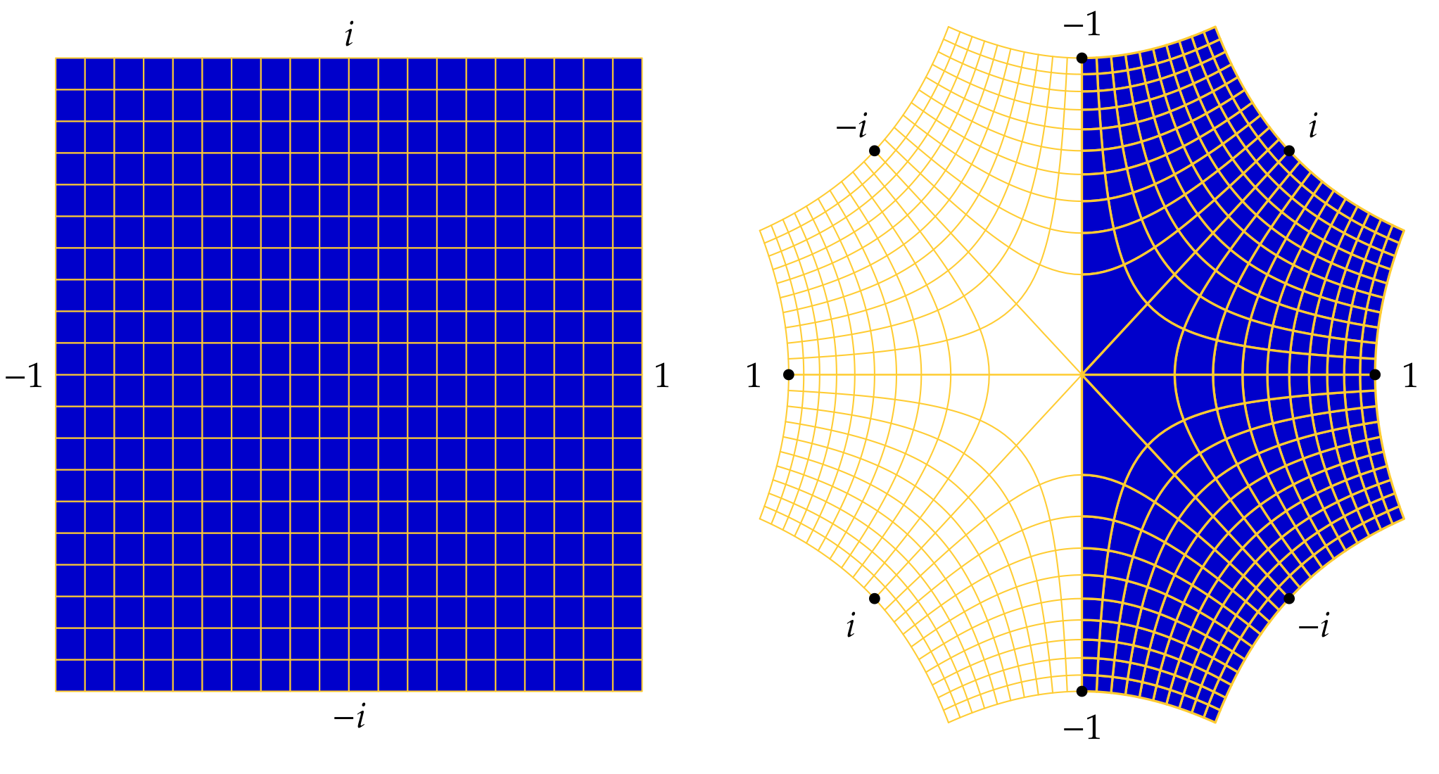
Though we cannot graph the total square root any more than we can properly graph the principal square root, we can plot the \(w\)-plane and \(z\)-plane side by side:
The labels are values of \(w\). In the right-hand diagram a label \(w\) is placed at each point \(z\) of \(\Sqrt(w)\). The shaded half-plane on the right depicts the principal square root. The discontinuities are made visible by the presence of two “\(-1\)” labels. This graph, perhaps better than any other, conveys how the principal square root slits the plane along the non-positive axis and “opens up” this ray into the imaginary axis.
The Riemann Surface of Square Root
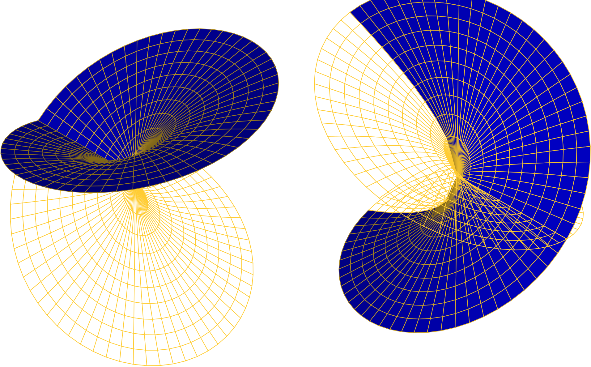
Instead of allowing the square root to take two values at each non-zero complex number \(w\), we can enlarge the domain, creating two points for each \(w\).
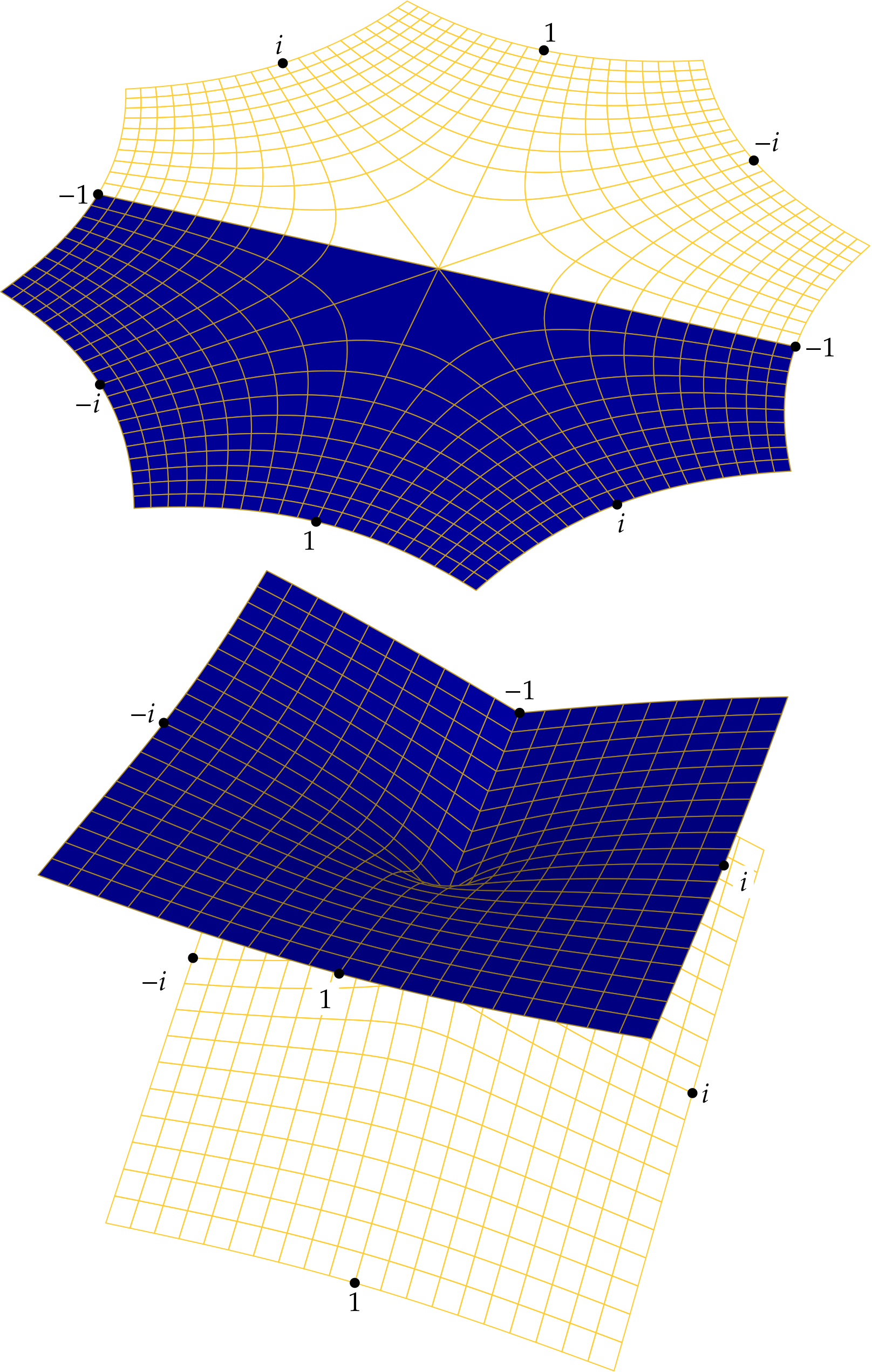
The diagram shows the “unwrapped” \(z\)-plane and “wrapped” \(z\)-plane, which sits over the \(w\)-plane (not shown). Under squaring, each half of the \(z\)-plane (containing the octagon) maps onto the complex plane. In the lower picture, showing the Cartesian plot of the complex parabola, we use vertical position to keep track of the two “copies” of the image. Vertical projection of the bottom object doubly-covers the \(w\)-plane, effecting the squaring mapping.
In four-space, the unwrapped octagon can be smoothly deformed into the two-sheeted covering at bottom. To those of us constrained to live in three-space, it's easier to imagine slitting the octagon along a ray from the origin, doubling all angles at the center to wrap twice around \(0\), then re-gluing the edges of the slit, obtaining the bottom picture.
The plane containing the octagon, or equivalently the two-sheeted object, is the Riemann surface of the square root. On its Riemann surface, the square root is a single-valued function: Effectively, \(z\) is the square root of \(w = z^{2}\).
Conclusions
Our wish to extend the familiar parabola to the complex realm has taken us on an excursion. We have seen the subtlety and importance of domains and ranges of functions, of polar coordinates and the interplay between polar angles and continuity, of algebra (which allows us to work easily with four-space) and geometry (which motivates discarding a coordinate and helps us interpret the results).
Why are we not compelled to pursue these considerations over the reals? Briefly, the two real branches of square root are separated by the origin, where the tangent line is vertical. When we look at inverse trig functions, the same barrier occurs: Either we encounter a vertical tangent when we pass between branches (as with \(\arcsin\)), or distinct branches are separated (as with \(\arctan\)). In the complex plane, however, a single point is no barrier: We can travel in a loop around a point. When we do this, keeping track of the value of some continuous function, we may find the value has changed, as if we were asking about our altitude while circling in a parking garage.
Calculus over the complex numbers must grapple with multi-valued functions. The square root is arguably the simplest example, yet it exhibits qualitative behavior shared by “branch points” and “multi-sheeted Riemann surfaces” that naturally arise when we attempt to invert a complex-differentiable function in a neighborhood of a critical point. If your appetite is whetted, you may enjoy similarly analyzing cube roots, or general \(n\)th roots!