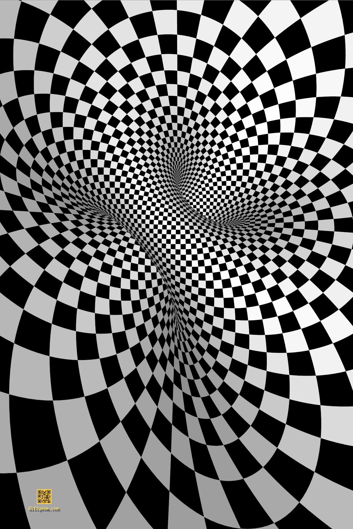
The poster and T-shirt design Cyclide Check depicts a checkerboard pattern on a parabolic cyclide, a type of torus with one point at infinity.
In various writings I've described mathematics as a landscape. That metaphor is as good as any here. Cyclide Check is a destination, but at first glance it's atop a precipice. How could anyone possibly get there? In mathematics as in hiking, the answer involves extended exploring, learning the terrain, following paths with attention.
Ingredients
Constructive laziness was a common refrain in my undergraduate classrooms. Let's make our way to the checkered cyclide using only school mathematics, but assembled in ways not usually seen in school.
The Complex Coordinate Plane
Algebraically, we'll work with ordered pairs of complex numbers, \((z, w)\). When resolving into real and imaginary parts is convenient, we'll write \(z = x + iy\), \(w = u + iv\), and identify \((z, w) \sim (x, y, u, v)\).
Geometrically, we're working in \(4\)-space. The “complex coordinate axes” are the sets \((z, 0)\) where \(w = 0\) and \((0, w)\) where \(z = 0\). Each complex axis is a real plane, and these axes meet in one point, \((0, 0)\), where \(z = w = 0\). The fact of two planes intersecting at one point may seem strange, but \(4\)-space has more room than \(3\)-space. Further, the complement of each complex axis is connected, just as a plane with one puncture is connected.
Our complex coordinate plane comes equipped with multiplication by complex scalars. If \(c\) is complex, then \(c \cdot (z, w) = (cz, cw)\). The origin \((0, 0)\) is fixed by scalar multiplication.
Inversely, if \((z, w) \neq (0, 0)\), then under scalar multiplication \((z, w)\) sweeps out the complex line (special type of real \(2\)-plane) containing \((0, 0)\) and \((z, w)\). Further, we have \(c \cdot (z, w) = c’ \cdot (z, w)\) if and only if \((c – c’) \cdot (z, w) = (0, 0)\), if and only if \(c = c’\).
Exercise 1: If \((z, w)\) and \(z’, w’)\) are non-zero pairs, then there exists a non-zero complex number \(c\) such that \(c \cdot (z, w) = (z’, w’)\) (one point is a scalar multiple of the other) if and only if \(zw’ = wz’\) (both points lie on a complex line through \((0, 0)\)).
The Unit Sphere
The (hypotenuse) distance from \((0, 0)\) to \((z, w)\) is \[ \bigl(|z|^{2} + |w|^{2}\bigr)^{1/2} = \sqrt{x^{2} + y^{2} + u^{2} + v^{2}}. \] The unit sphere is the set of points at distance \(1\) from \((0, 0)\), namely the set of \((z, w)\) such that \(|z|^{2} + |w|^{2} = 1\).
If \(t\) is a unit complex number and \((z, w)\) is a point of the unit sphere, then \((tz, tw)\) is a point of the unit sphere since \[ |tz|^{2} + |tw|^{2} = |t|^{2}\bigl(|z|^{2} + |w|^{2}\bigr) = 1. \] Geometrically, each point of the unit sphere determines a unique circle swept out by scalar multiplication. This circle lies on a complex line through the origin, hence has radius \(1\). In other words, under scalar multiplication each point on the unit sphere traces a great circle.
Exercise 2: If \(t\) is a unit complex number, show that its complex conjugate \(\bar{t}\) is its reciprocal \(1/t = t^{-1}\). If in addition \((z, w)\) is a point of the unit sphere, show \((tz, \bar{t}w)\) is a point of the unit sphere.
Product Tori
Assume \(a\) and \(b\) are positive real numbers. The condition \(|z| = a\) defines the circle of center \(0\) and radius \(a\) in the \(z\) plane. The condition \(|w| = b\) similarly defines the circle of center \(0\) and radius \(b\) in the \(w\) plane. The two conditions together define an ordered product of circles in the complex coordinate plane, namely a product torus.
If \(a^{2} + b^{2} = 1\), our product torus is a subset of the unit sphere. (Why?) Further, scalar multiplication by a unit complex number maps our torus to itself: If \(|z| = a\) and \(|w| = b\), then \(|tz| = a\) and \(|tw| = b\).
Our product torus may be viewed as sweeping a circle of radius \(a\) around a circle of radius \(b\). These “small” circles correspond to the familiar “longitudes” and “latitudes” on a circular torus in \(3\)-space. As we saw earlier, however, the “circular orbits” swept by scalar multiplication are great circles, of radius \(1\); consequently, they are neither longitudes nor latitudes. What are these circles? To answer this question, we'll approach from another angle, as it were.
If \(r\) denotes a real number, the complex path \(A(r) = ae^{ir} \sim (a\cos r, a\sin r)\) traces the circle \(|z| = a\) with speed \(a\). Each real interval of length \(2\pi\) wraps once around this circle.
Similarly, if \(s\) is real, the complex path \(B(s) = be^{is} \sim (b\cos s, b\sin s)\) traces the circle \(|w| = b\) at speed \(b\). Each real interval of length \(2\pi\) wraps once around this circle.
Taking the ordered product of these paths, we get the mapping \[ f(r, s) = (ae^{ir}, be^{is}) \sim (a\cos r, a\sin r, b\cos s, b\sin s) \] from the real \((r, s)\) plane to the complex \((z, w)\) plane. The image is our torus, \(|z| = a\) and \(|w| = b\). Each axis-oriented \(2\pi \times 2\pi\) square in \((r, s)\) wraps once around the torus, and the mapping \(f\) “glues” the opposite sides with consistent orientation.
To see the circles swept by scalar multiplication, let \(\theta\) denote a polar angle and write \(t = e^{i\theta}\). The law of exponents, a.k.a., the sum-of-angles formulas for the circular functions, gives \[ t \cdot (z, w) = e^{i\theta} \cdot (ae^{ir}, be^{is}) = (ae^{i(r+\theta)}, be^{i(s+\theta)}). \] Geometrically, rotating both complex axes by \(\theta\) translates \((r, s)\) to \((r + \theta, s + \theta)\).
In other words, vertical lines \(r = \text{constant}\) and horizontal lines \(s = \text{constant}\) map (under \(f\)) to longitudes and latitudes of our torus. (We cannot say which is which, because on our torus in the complex coordinate plane there is no clear distinction! Latitudes and longitudes are a “broken symmetry” upon mapping the torus to real \(3\)-space.) Diagonal lines of slope \(1\), by contrast, map to our great circles on the torus.
Exercise 3: In Exercise 2 you found another family of great circles on the torus. To which curves in \((r, s)\) do those correspond?
Retrieving the Torus
Our product torus sits in real \(4\)-space. In order to see it, we'd like to map it to \(3\)-space, which better conforms to our spatial surroundings and intuition.
Our technique will be stereographic projection: Think of (“our”) real \(3\)-space as the set \(v = 0\) with rectangular coordinates \((x, y, u) \sim (x, y, u, 0)\). Place a point “light source” at \((0, 0, 0, 1)\), one of two points on the unit sphere at maximum distance from our “equatorial” universe. (What are the coordinates of the other?) Each point \((x, y, u, v)\) such that \(v < 1\) casts a “shadow” in our universe, the location where the ray from \((0, 0, 0, 1)\) through \((x, y, u, v)\) hits the equator where \(v = 0\). By similar triangles or vector algebra, this location is \[ \Pi(x, y, u, v) = \frac{1}{1 - v}(x, y, u, 0). \] For example, the point \(f(r, s) = (a\cos r, a\sin r, b\cos s, b\sin s)\) on our torus maps to \[ (\Pi \circ f)(r, s) = \frac{1}{1 - b\sin s}(a\cos r, a\sin r, b\cos s, 0). \] (Remember: \(a^{2} + b^{2} = 1\) and we are assuming both \(a\) and \(b\) are positive.) You may enjoy plotting this parametric surface and verifying it is a circular torus, though probably not the parametrization you saw in calculus.
Describing a checkerboard torus is now straightforward: Use diagonal lines of slope \(\pm 1\) to divide the axis-oriented square \([-\pi, \pi] \times [-\pi, \pi]\) (say) into diamonds and right isosceles triangles. Color these alternately black and white like a tiled floor, and apply the preceding mapping with \(a = b = 1/\sqrt{2}\).
Smooth Cyclides
There is one more step to get the surface in Cyclide Check. We rotate our torus and see what happens to the “stereographic shadow” in \(3\)-space, particularly when our rotated torus passes through the “light source” \((0, 0, 0, 1)\).
Without going too far into linear algebra, how should we think geometrically of “rotation” in \(4\)-space? The key insight from planar and spatial intuition is that “rotation (about the origin)” moves some plane and fixes everything through the origin and orthogonal to that plane.
Exercise 4: In \(4\)-space, how many planes contain two real coordinate axes? How many of these planes are “suitable” for rotating our torus to pass through the light source at \((0, 0, 0, 1)\)?
We'll rotate the “imaginary” plane containing the second and fourth axes, keeping the orthogonal “real” plane (containing the first and third axes) fixed. Let's use \(R_{\theta}\) to denote rotating the plane of the second and fourth axes by \(\theta\). In real coordinates, this rotation is given by the formula \[ R_{\theta}(x, y, u, v) = (x, y\cos\theta – v\sin\theta, u, v\cos\theta + y\sin\theta). \] Since \[ f(r, s) \sim (a\cos r, a\sin r, b\cos s, b\sin s), \] our rotated torus has parametrization \[ (R_{\theta} \circ f)(r, s) \sim (a\cos r, a\sin r \cos\theta – b\sin s \sin\theta, b\cos s, b\sin s \cos\theta + a\sin r \sin\theta). \] Stereographically projecting gives the parametrization \[ (\Pi \circ R_{\theta} \circ f)(r, s) \sim \frac{(a\cos r, a\sin r \cos\theta – b\sin s \sin\theta, b\cos s)}{1 – (b\sin s \cos\theta + a\sin r \sin\theta)}. \]
The interactive program Morph lets you investigate a handful of surfaces in \(4\)-space and \(6\)-space. To visualize this torus, select “cyclide” from the drop-down menu. Use the arrow keys to rotate the surface in \(3\)-space; use comma and period (less-than and greater-than) to change the rotation angle in \(4\)-space. Particularly, you can see how longitudes and latitudes are exchanged when the torus rotates through the light source.
Since \(r\) and \(s\) were rectangular coordinates for our product torus, we need to adjust them to get the “diamond” tiling. An easy tweak is to replace \(r\) by \(r + s\) and \(s\) by \(r – s\), which gives the parametrization \[ F(r, s) = \frac{\bigl(a\cos(r + s), a\sin(r + s) \cos\theta – b\sin(r – s) \sin\theta, b\cos(r – s)\bigr)}{1 – (b\sin(r – s) \cos\theta + a\sin (r + s) \sin\theta)}. \]
To investigate this coordinate system in Morph, select “twistor torus” from the drop-down menu.
The preceding formula is simple and explicit, but not likely to be written down by casual inspection. The formula also contains three parameters: \(a\), \(b\), and \(\theta\); how should these be chosen?
Remember that \(a\) and \(b\) are positive and \(a^{2} + b^{2} = 1\). To get a square torus amounts to assuming \(a = b\); thus \(a = b = 1/\sqrt{2}\), as noted earlier. With this choice, multiplying and dividing our parametrization by \(\sqrt{2}\) gives \[ (\Pi \circ R_{\theta} \circ f)(r, s) \sim \frac{(\cos r, \sin r \cos\theta – \sin s \sin\theta, \cos s)}{\sqrt{2} – (\sin s \cos\theta + \sin r \sin\theta)}. \] Ensuring our rotated torus passes through \((0, 0, 0, 1)\) amounts to ensuring the denominator vanishes for some choice of \((r, s)\), namely, to ensuring \[ \sin s \cos\theta + \sin r \sin\theta = \sqrt{2} \] has a solution \((r, s)\). Each of \(\sin r\) and \(\sin s\) is no larger than \(1\), and \(\cos\theta + \sin\theta\) is no larger than \(\sqrt{2}\), with equality if and only if \(\theta = \pi/4\). (To see this geometrically, consider lines of slope \(-1\) in the plane, along which \(x + y\) is constant. The “most northeast” such line, which maximizes \(x + y\), touches the unit circle where \(x = y = 1/\sqrt{2}\).)
Needing to rotate our torus by \(1/8\) of a turn (\(45\) degrees) makes geometric sense: The square torus intersects the \((y, v)\)-plane (where \(x = u = 0\)) in four points, the vertices of a square. Rotating this square \(45\) degrees places one of these points at the light source.
Answers to Exercises
Exercise 1: If there exists a \(c\) such that \(c \cdot (z, w) = (z’, w’)\), then \(z’ = cz\) and \(w’ = cw\), so \(zw’ = z(cw) = (cz)w = z’w\).
Conversely, assume \(zw’ = z’w\). If \(w \neq 0\), then set \(c = w’/w\). We have \(cz = zw’/w = z’w/w = z’\) and \(cw = w’\). If instead \(w = 0\), then \(z \neq 0\) since \((z, w) \neq (0, 0)\). If we set \(c = z’/z\), then \(cz = z’\) and \(cw = z’w/z = zw’/z = w’\).
Exercise 2: If \(t\) is a unit complex number, namely \(|t| = 1\), then \(1 = |t|^{2} = t\bar{t}\), so \(\bar{t} = 1/t\). Further, \(\bar{t}\) is a unit complex number. If \((z, w)\) is on the unit sphere, then \[ |tz|^{2} + |\bar{t}w|^{2} = |z|^{2} + |w|^{2} = 1, \] so \((tz, \bar{t}w)\) is on the unit sphere.
Exercise 3: The multiplication in Exercise 2 adds to one angle variable and subtracts from the other; the resulting circles correspond to lines of slope \(-1\) in the \((r, s)\)-plane.
Exercise 4: There are six coordinate planes in \(4\)-space because there are six ways to pick two objects from a set of four. (We may select any of four axes, then any of three distinct axes, for a total of \(12\) choices. Each coordinate plane comes from precisely two such choices. For example, the \((2, 4)\) and \((4, 2)\) coordinates planes are the same. Consequently, there are \(12/2 = 6\) distinct coordinate planes.
In order to rotate our torus to the light source, our rotation must involve the fourth axis. Further, the \((3, 4)\) coordinate plane, namely the \(w\)-axis, is not suitable: rotating the \(w\)-axis preserves our product torus as a set. Only two planes are “suitable”: \((1, 4)\) and \((2, 4)\). We picked \((2, 4)\) arbitrarily, but with only two options rather than six.