Rays and Perspective
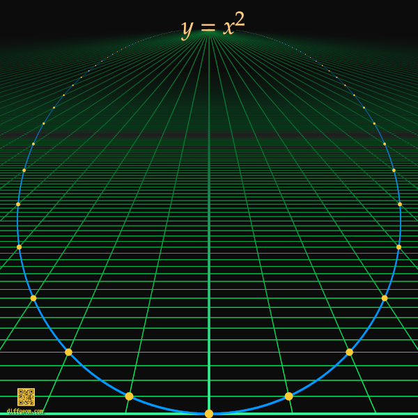
Imagine a flat floor extending to infinity in all directions and covered with square tiles, creating a Cartesian coordinate system. A parabola, such as the graph \(y = x^{2}\), is painted on the floor. If we stand below the origin and look at the parabola in perspective, what kind of curve do we see? To answer this question, we first need to think about the geometry of vision, and what we mean by a picture.
A simple model for perspective vision starts with a point \(O\) in space modeling an eye. A half-line starting from \(O\) models a ray of light into the eye, and indeed geometers usually call such half-lines rays from \(O\). Two points in space lying on a ray from \(O\) appear at the same location, with the nearer point blocking the farther. In other words, a ray from \(O\) models a point seen by \(O\). The set of all rays forms the field of view from \(O\).
The set of rays from \(O\) may be identified with the unit sphere \(S\) centered at \(O\): Every ray from \(O\) hits the unit sphere exactly once, and every point of the unit sphere determines a unique ray from \(O\). We might think of the sphere as a movie screen onto which objects of three-space are radially projected (i.e., along rays), and a "picture" as a piece of the sphere with images of objects. A planetarium dome is a hemisphere on which the night sky can be projected.
In practice, a "picture" is usually a flat rectangle, such as a painting, drawing, photograph, or computer screen. Imagine looking through a window with one eye closed, and tracing objects you see on the glass. The mathematician C. F. Gauss discovered in the 1800s that a spherical region cannot be mapped to a plane region while preserving all distances between points. Nonetheless, our brains can interpret such tracings as outlines of three-dimensional scenes.
Mathematically, an arbitrary plane \(P\) not passing through \(O\) models a screen on which a viewer at \(O\) sees the contents of space. Each point of \(P\) determines a ray from \(O\). Not every ray from \(O\) hits \(P\), however: The rays from \(O\) that hit \(P\) fill an open hemisphere of \(S\). The "equator" bounding this open hemisphere consists of rays from \(O\) parallel to \(P\). These are in a sense "arbitrarily close to" rays that do hit \(P\), and may be viewed as representing points "at infinity in \(P\), as seen by \(O\)."
By making a sneaky observation, we can see what a parabola looks like when viewed from above its plane. A parabola is a conic section, the intersection of a plane and a right circular cone. By picking the cone appropriately, we may assume the plane of the parabola is the sectioning plane. If we place our eye at the vertex, we see a perfect circle tangent to the horizon!
If we place our eye at a different point, we can shear-transform the cone in a way that preserves the plane of the parabola but moves the vertex to the new location of our eye. The transformed cone generally has elliptic cross section, so we see the parabola as an ellipse, but still tangent to the horizon.
Projective Spaces
For technical reasons, working with lines through \(O\) is mathematically preferable to working with rays. Briefly, lines make geometric and algebraic sense in more generality than rays. In more detail, lines are defined for all number systems (or "fields" as they are known to mathematicians), while rays are only defined when we work with "ordered fields" having a concept of less-than. The real number system is ordered, but other important number systems, such as the complex numbers or residue classes of integers, are not. Motivated by the geometry of perspective, we call the set of lines through the origin in a Cartesian space a projective space. Our pictures will be drawn for the real number system, but the concepts below make sense in the complex numbers, and over other fields, as well.
The Projective Line
Because we can represent the real plane on a flat sheet of paper, we might expect we can represent the set of lines through the origin by a picture. A line through the origin is determined by one real parameter, such as polar angle, or slope. This means the set of lines is itself "line-like" or one-dimensional. We call the set of lines through the origin in the plane the (real) projective line. To "represent the projective line" we seek a plane curve whose points correspond to lines through the origin.
In parallel to the situation with rays, we might look at the unit circle. Each line through the origin hits the circle in a pair of diametrically opposite points. The unit circle itself is therefore not itself a representation of the real projective line, though it is close: The set of antipodal pairs on the unit circle corresponds to the real projective line. This observation is useful (and generalizes, as we will see), but does not quite fulfill our aim to represent the projective line as a plane set of points.
As a second attempt, we might consider a line not passing through the origin, perhaps the vertical line with Cartesian equation \(x = 1\). Every non-vertical line through \((0, 0)\) has equation \(y = mx\) for a real number \(m\), the slope, and each such line hits \(x = 1\) at the point \((x, y) = (1, m)\), where \(x = 1\) and \(y = mx = m\). This vertical line therefore represents "most" of the real projective line. There is precisely one "missing" line, the vertical axis through \(O\).
As suggested in the diagram above, there is a way to blend the chocolate of the unit circle with the peanut butter of the vertical line \(x = 1\): Consider a circle passing through the origin, such as the circle of radius \(\frac{1}{2}\) with center \((\frac{1}{2}, 0)\). Every non-vertical line through \(O\) hits this circle in two distinct points, one of which is the origin itself. The "other" point, not the origin, corresponds to our line through \(O\). What about the vertical line through \(O\)? This line is tangent to the circle at the origin. In a sense that can be made precise using either algebra or calculus, the tangent line also "intersects the circle twice": Once at the origin, and again at the origin! For the vertical line, the "other" point is the origin.
In this way, points of our circle through the origin correspond precisely with lines through the origin. Incidentally, there is nothing unique about this particular circle; an arbitrary circle through the origin, no matter how large or small in radius and no matter what tangent line at \(O\), similarly represents the real projective line. Further, plenty of non-circular curves also represent the real projective line. Circles just happen to be geometrically nice.
Recall polar coordinates \((r, \theta)\) in the plane: \(r\) is distance from \(O\) and \(\theta\) is angle measured counterclockwise from the positive horizontal ray. The unit circle, the vertical line \(x = 1\), and the circle with radius \(\frac{1}{2}\) and center \((\frac{1}{2}, 0)\) have remarkable representations in polar coordinates. The unit circle has equation \(r = 1\): The distance from the origin to a point on the unit circle is \(1\) regardless of polar angle! To describe the vertical line in polar coordinates, recall the polar-to-Cartesian conversion formula \(x = r\cos\theta\). The line \(x = 1\) has polar equation \(r\cos\theta = 1\), or \(r = 1/\cos\theta = \sec\theta\). This is undefined when \(\cos\theta = 0\), which occurs when \(\theta\) determines a vertical polar ray. Geometrically, polar coordinates "see" the missing point of the projective line, assigning an angle perpendicular to the horizontal.
What about the small circle? It turns out this circle has polar equation \(r = \cos\theta\)! To justify this claim, recall that the circle with radius \(R = \frac{1}{2}\) and center \((x_{0}, y_{0}) = (\frac{1}{2}, 0)\) has Cartesian equation \((x - x_{0})^{2} + (y - y_{0})^{2} = R^{2}\). Substituting the known radius and center gives \[ (x - \tfrac{1}{2})^{2} + y^{2} = (\tfrac{1}{2})^{2}. \] Expanding, \(x^{2} - x + \frac{1}{4} + y^{2} = \frac{1}{4}\). Rearranging and canceling give \[ x^{2} + y^{2} - x = 0. \] In polar coordinates, \(x^{2} + y^{2} = r^{2}\) and \(x = r\cos\theta\), so the equation of our circle may be written \[ r(r - \cos\theta) = r^{2} - r\cos\theta = 0. \] It suffices to show this polar equation has the same Cartesian solution set as \(r - \cos\theta = 0\), or \(r = \cos\theta\). If \((r, \theta)\) satisfies \(r - \cos\theta = 0\), then certainly \(r(r - \cos\theta) = 0\). Inversely, if \(r(r - \cos\theta) = 0\), then either \(r - \cos\theta = 0\) and we are done, or \(r = 0\) and our Cartesian point is the origin. But the origin lies on the polar graph \(r - \cos\theta = 0\), so again we are done.
This algebraic argument expresses the geometric fact that every line through the origin hits the small circle twice: Once where \(r = 0\) (at the origin) and once where \(r = \cos\theta\) (a point of the small circle that may or may not be the origin).
This picture of the real projective line is as nice as we could hope. Unfortunately, the picture is almost misleadingly nice. Over the complex numbers, the picture is only metaphorically correct. The complex Cartesian plane is a real four-dimensional space. The unit sphere, analogous to the unit circle above, is "three-dimensional": smoothly specifying points on the sphere requires three real parameters. The vertical complex line is a real plane. It turns out the complex projective line is a real sphere like a soap bubble, but the "projection" from the unit sphere to the projective line is more complicated than identifying pairs of antipodal points. Instead, multiplication by complex scalars of magnitude \(1\) effects the Hopf action on the unit sphere. The Hopf action causes each point of the unit sphere to trace a great circle, or Hopf fiber. Each Hopf fiber corresponds to a unique point of the complex projective line. The complex projective line itself, however, does not naturally sit inside the complex Cartesian plane.
The Projective Plane
Our picture of the real projective line also does not perfectly generalize to higher dimensions, though the situation is a bit better than for the complex projective line. Suppose we replace the real plane with real Cartesian three-space, we replace the unit circle with the unit sphere, and we replace the line \(x = 1\) with the plane \(z = 1\). (The use of \(z\) instead of \(x\) is for convenience, allowing us to keep using \(x\) and \(y\) as something like plane coordinates.) Let's see what generalizes.
Each line through \(O\) hits the unit sphere in a pair of diametrically opposite points, i.e., a pair of antipodes. Inversely, each antipodal pair determines a unique line through \(O\). The set of lines through the origin, or real projective plane, may be viewed as the set of antipodal pairs on the unit sphere.
Suppose \(\ell\) is a line through the origin that does not lie in the horizontal plane \(z = 0\). Then \(\ell\) intersects the plane \(z = 1\) in a unique point. In a precise sense, "most" lines in space do not lie in the plane \(z = 0\). Unlike the situation in the plane, however, there are infinitely many "missing" lines in the plane \(z = 0\). Let's explore the geometric significance of these missing lines.
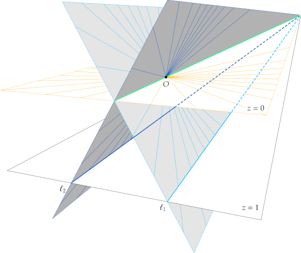
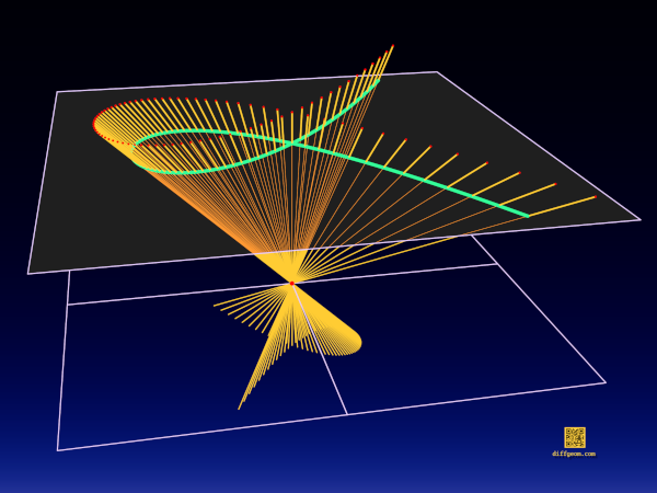
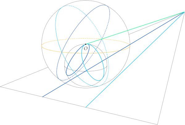
In the diagram, space is oriented so the plane \(z = 1\) lies below \(O\), as if seen from the air. The plane \(z = 0\) is parallel to \(z = 1\) in three-space. Because a projective point is a line through \(O\) in Cartesian space, each projective line in the plane \(z = 1\) corresponds to a plane through \(O\). Two projective lines are shown, labeled \(\ell_{1}\) and \(\ell_{2}\). Let \(P_{1}\) be the light gray plane containing \(\ell_{1}\) and \(O\). Let \(P_{2}\) be the medium-gray plane containing \(\ell_{2}\) and \(O\).
Here is the crucial geometric point (as it were): The planes \(P_{1}\) and \(P_{2}\) are distinct and both contain \(O\). Consequently, they intersect in a line through \(O\). But a line through \(O\) is a projective point! In words, any two distinct projective lines in the Euclidean plane \(z = 1\) intersect in a unique projective point.
If \(\ell_{1}\) and \(\ell_{2}\) are not parallel in \(z = 1\), the fact of their intersecting is no surprise. But what if the projective lines \(\ell_{1}\) and \(\ell_{2}\) are parallel? Parallel lines do not meet, so our projective lines do not intersect in the Euclidean plane \(z = 1\). Where, then, is their projective point of intersection? As the diagram shows, if \(\ell_{1}\) and \(\ell_{2}\) are parallel, then the planes \(P_{1}\) and \(P_{2}\) meet in a line through \(O\) and parallel to both \(\ell_{1}\) and \(\ell_{2}\). That is, the planes meet along a line in the plane \(z = 0\). The corresponding projective point is "missing" from the plane \(z = 1\). As we will see momentarily, it is reasonable to view the missing projective points as lying "at infinity" in the Euclidean plane \(z = 1\).
To restate our conclusions so far: Parallel Euclidean lines \(\ell_{1}\) and \(\ell_{2}\) in the plane \(z = 1\) intersect at a projective point not in \(z = 1\). This projective point is represented by the unique line \(\ell_{0}\) in the plane \(z = 0\) that is parallel to \(\ell_{1}\) and \(\ell_{2}\). This projective point corresponds to the common direction of \(\ell_{1}\) and \(\ell_{2}\).
Suppose \(p\) is a point of the plane \(z = 1\), and \(\ell = Op\) is the line through \(O\) and \(p\). How can we move \(p\) to make \(\ell\) "approach" the line \(\ell_{0}\) in the plane \(z = 0\)? As should be visually plausible, the farther we move \(p\) along a line parallel to \(\ell_{0}\), the closer \(\ell\) is to \(\ell_{0}\). In this limiting sense, the projective point represented by \(\ell_{0}\) lies at infinity along every projective line parallel to \(\ell_{0}\) in the plane \(z = 1\).
Qualitatively, the projective plane contains a "finite plane" \(z = 1\) with Euclidean geometry, and a projective line \(z = 0\) "at infinity" whose projective points correspond to directions in the plane \(z = 1\), one direction for each family of parallel projective lines. Any two parallel projective lines in \(z = 1\) meet at infinity, at the projective point corresponding to their common direction. When everything clicks, this picture is beautifully tidy!
In the diagram, the parallel lines \(\ell_{1}\) and \(\ell_{2}\) visibly intersect. Our brains, accustomed to straight roadways and railroad tracks, interpret the intersection as being infinitely far away. At the same time, the point of intersection lies as a definite finite position in the plane of the diagram. Probably without thinking twice, we see and accept the same phenomenon any time we encounter parallel lines in a painting or photograph. The mathematical point, however, is important to emphasize: A particular projective point is a line \(\ell\) through \(O\). Whether \(\ell\) is "in the finite plane" or "at infinity" is not an attribute of \(\ell\) alone, but depends on the choice of finite plane.
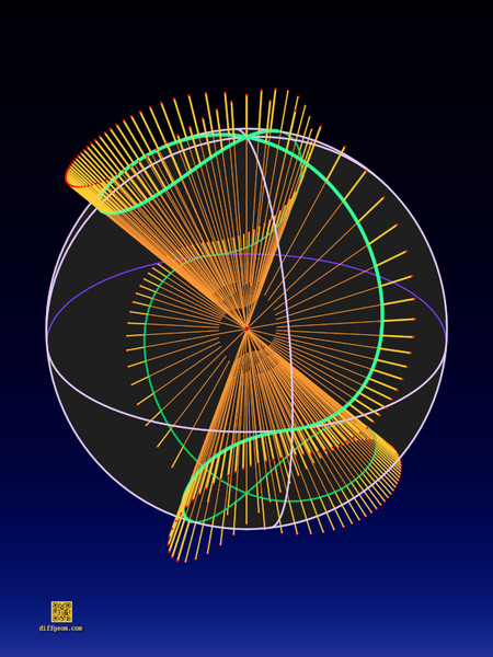
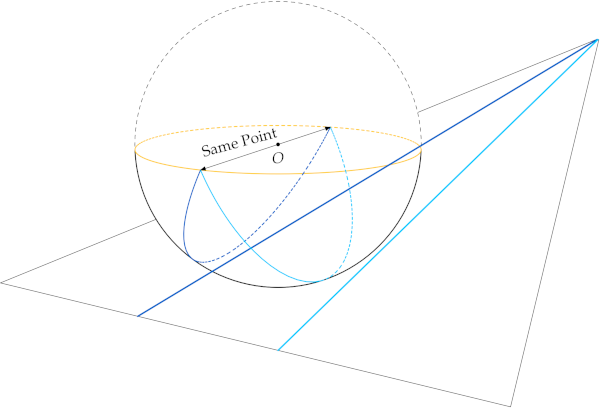
Alternatively to picking a finite plane and a projective line at infinity, we can visualize the real projective plane in terms of the unit sphere. On the unit sphere, the previous diagram looks like this:
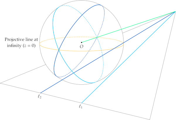
Each projective line corresponds to a plane containing \(O\) in Cartesian three-space. Every such plane cuts the unit sphere in a great circle. Two great circles on the sphere intersect in a pair of antipodal points, i.e., in a projective point. When we pick a finite plane such as \(z = 1\), the parallel plane through \(O\) represents the projective line at infinity, \(z = 0\). Our two parallel projective lines visibly meet on the projective line at infinity, at the projective point represented by the light green line.
The "finite plane" and "unit sphere" descriptions of the projective plane are complementary. One advantage of referring to the unit sphere is linguistic. Earlier we had to speak carefully of projective points, which are (or are represented by) lines in Cartesian three-space; we had to speak of projective lines, which are planes in Cartesian three-space. There is a dimensional mismatch that we took pains to clarify with each usage. Radially projecting Cartesian three-space (with \(O\) removed) to the unit sphere "projects away" a dimension, "repairing" the dimensional mismatch. On the sphere, a "projective point" is two antipodal points; a "projective line" is a great circle. We can drop some of our pedantry and speak of "points" and "lines" without ambiguity.
Further, while it may seem suspicious to say "parallel lines meet at infinity," it is easy to see that any two great circles intersect in a pair of antipodal points. That is, the sphere picture makes clear that any two projective lines intersect.
One related benefit of the sphere is perceptual: We can see the entire sphere at once. A plane, by contrast, necessarily extends outside every viewing window, and may in addition have a horizon. Looking at the sphere probably makes clearer that there is no "funny business" at infinity, no possibility of a point escaping to infinity where we cannot see it.
As noted earlier, the planar picture of the projective line does not generalize nicely to the projective plane. Let's see why. If we consider a sphere \(S\) through \(O\) analogously to a circle through \(O\), then "most" lines through \(O\) do hit \(S\) in two distinct points. The exceptions are lines tangent to the sphere at \(O\). The problem is, there are now infinitely many tangent lines, not merely one, and in this scheme all correspond to a single point of \(S\). In a sphere through \(O\), the projective line represented by the plane tangent to \(S\) at \(O\) is "squeezed" to a point.
Instead, let's start with the unit sphere and "carve away" as much as we can, i.e., remove one point from as many antipodal pairs as possible. After a bit of thought, we can remove an open hemisphere (excluding the boundary circle, such as the northern hemisphere as shown below), leaving a closed hemisphere (including the boundary circle, the southern hemisphere as shown). Every line through \(O\) hits the closed southern hemisphere at least once; lines in the plane of the boundary circle (the equator) hit the hemisphere twice. In the diagram below, the open southern hemisphere corresponds to a finite Euclidean plane. Lines are now half-arcs of great circles ending on the equator. The equator is the line at infinity relative to the finite plane of the southern hemisphere. To get a representation of the projective plane, we must identify (or "glue together") antipodal pairs on the boundary. One pair is shown. To complete the gluing, we need to "wrap the equator around itself twice" so that every point is glued to its antipode.
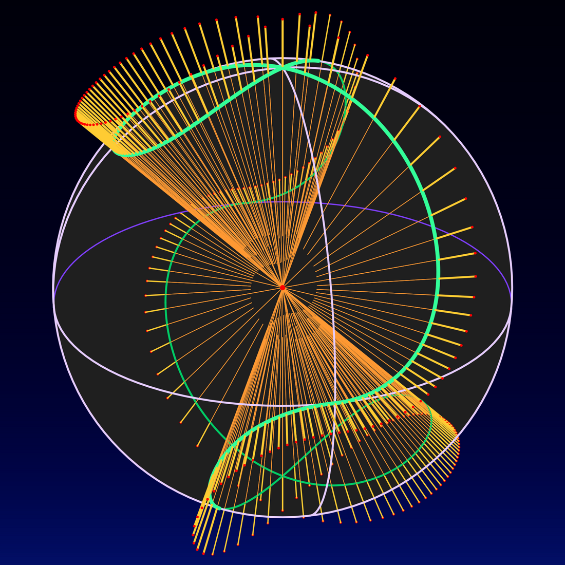
This sounds difficult, and indeed, a non-trivial theorem of algebraic topology says the resulting abstract surface cannot be topologically represented ("embedded") in Cartesian three-space. On the other hand, this abstract surface can be represented ("smoothly immersed") if we allow self-intersections. Our Luminography prints illustrate one way to accomplish the immersion. The animation loop below shows images of concentric circles under the Bryant-Kusner immersion of the projective plane, purple near the center and bright green approaching the boundary. Successive circles, lit frame by frame, become increasingly triangular; the triangles' corners each undergo a half-twist and pass through themselves, yielding a trefoil knot; a trefoil is the boundary of a Möbius band, and as the band narrows the boundary approaches the central circle traced twice, effecting the antipodal gluing at the boundary.
Homogeneous Coordinates
My emphasis at the Differential Geometry math art shop is shape. If you try to learn more about projective geometry, however, you'll quickly run into algebra and formulas. Here is a capsule introduction to projective coordinates.
A point of Cartesian space may be viewed as an ordered triple \((x, y, z)\). Each point of projective space corresponds to a triple different from \((0, 0, 0)\). Two non-zero triples represent the same projective point precisely when each is a scalar multiple of the other. For instance, \((4, 0, -3)\) and \((8, 0, -6)\) and \((-4, 0, 3)\) represent a single projective point. Generally, in this example, \((4t, 0, -3t)\) represents a single projective point regardless of \(t \neq 0\).
The ordered triple \((4, 0, -3)\) represents a point of Cartesian space. To distinguish the corresponding projective point, we write \([4 : 0 : -3]\). The colons signify ratios, and the square brackets connote "equivalence classes" where a single entity has multiple symbolic representations. The entries in a projective point \([x_{0} : y_{0} : z_{0}]\) are its homogeneous coordinates. At least one homogeneous coordinate must be non-zero; the expression \([0 : 0 : 0]\) does not signify a projective point.
If all three homogeneous coordinates are non-zero, we can make any particular coordinate equal to \(1\) by dividing. For instance, \begin{align*} [3 : -2 : 5] &= [1 : -\tfrac{2}{3} : \tfrac{5}{3}] && \text{divide each by \(3\)} \\ &= [-\tfrac{3}{2} : 1 : -\tfrac{5}{2}] && \text{divide each by \(-2\)} \\ &= [\tfrac{3}{5} : -\tfrac{2}{5} : 1] && \text{divide each by \(5\)}. \end{align*} Higher-dimensional projective geometry formally extends without difficulty, by lengthening the lists of homogeneous coordinates.
Projective mappings are invertible linear transformations of Cartesian space. These are conceptually not complicated, but when written out for the projective plane quickly become formidable-looking. On the projective line, projective mappings are also known as Möbius transformations. A general linear transformation has the form \[ \left[\begin{array}{@{}rr@{}} a & b \\ c & d \\ \end{array}\right]\left[\begin{array}{@{}r@{}} x \\ y \\ \end{array}\right] = \left[\begin{array}{@{}c@{}} ax + by \\ cx + dy \\ \end{array}\right],\quad ad - bc \neq 0. \] In the "finite part" of the projective line where \(y \neq 0\), we may divide homogeneous coordinates through by \(y\). Writing \(X = x/y\) and viewing columns as homogeneous coordinates, the previous transformation becomes \[ \left[\begin{array}{@{}rr@{}} a & b \\ c & d \\ \end{array}\right]\left[\begin{array}{@{}r@{}} X \\ 1 \\ \end{array}\right] = \left[\begin{array}{@{}c@{}} aX + b \\ cX + d \\ \end{array}\right] = \left[\begin{array}{@{}c@{}} (aX + b)/(cX + d) \\ 1 \\ \end{array}\right]. \] Briefly, this transformation has the form \(X \mapsto \dfrac{aX + b}{cX + d}\).
Our journey into the projective plane started with the parabola \(y = x^{2}\) and how this parabola looks to an observer above the \((x, y)\) plane. Earlier we gave a sneaky geometric answer. We can now approach the same question by algebra. Our first step is to homogenize the parabola's equation: Introduce a third variable \(z\), write the defining equation as a polynomial \(x^{2} - y = 0\) in two variables, and multiply each term by a power of \(z\) to make each term of the same degree: \[ x^{2} - yz = 0. \]
To motivate this process, note two things. First, in the plane \(z = 1\), every power of \(z\) has value \(1\), so the \(z\)-dependent factors we introduced disappear, leaving our original polynomial. Second, if a triple \((x, y, z)\) satisfies the homogeneous quadratic \(x^{2} - yz = 0\), and if \(t\) is a number, then \((tx, ty, tz)\) also satisfies the defining equation, since \[ (tx)^{2} - (ty)(tz) = t^{2}x^{2} - t^{2}yz = t^{2}(x^{2} - yz) = 0. \] Geometrically, we have taken the locus \(x^{2} - y = 0\), "suspended" it in the plane \(z = 1\), and given the equation of the generalized cone with vertex \(O\) described by the locus. This cone is by definition the union of lines through \(O\) and a point of our parabola, i.e., the representation of the parabola in the projective plane.
To see that the surface defined by \(x^{2} - yz = 0\) is projectively a circular cone, we can substitute \(y = u - v\) and \(z = u + v\), obtaining the equation \[ x^{2} - yz = x^{2} - (u - v)(u + v) = x^{2} - (u^{2} - v^{2}), \] or \(x^{2} + v^{2} = u^{2}\).
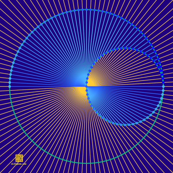
To give one more example of homogeneous coordinates, we'll examine the first image above, which depicts the "nodal cubic" \(x^{2}(x - 1) + y^{2} = 0\). Our homogenization procedure gives the equation \[ x^{3} - x^{2}z + y^{2}z = 0. \] To see what this curve looks like in the finite plane perpendicular to the \(x\)-axis, we set \(x = 1\), obtaining \[ 1 - z + y^{2}z = 0. \] We may rearrange to \(1 = (y^{2} - 1)z\), which lets us express \(z\) in terms of \(y\): \[ z = \frac{1}{y^{2} - 1}. \] To see what this curve looks like in the finite plane perpendicular to the \(y\)-axis, we instead set \(y = 1\) in the three-variable equation, obtaining \[ x^{3} - x^{2}z + z = 0. \] We may rearrange to \(x^{3} = (x^{2} - 1)z\), or \[ z = \frac{x^{3}}{x^{2} - 1}. \] These algebraic operations allow us to study the shape of a plane curve at infinity in a uniform way.
In retrospect, real projective plane geometry is little more than artistic perspective, the careful study of points, lines, and planes in Euclidean three-space. At the same time, "careful study" leads us quickly to unexpected territory, such as points at infinity where parallel lines meet, and paths that return to the finite realm after reaching and passing through infinity. Getting conceptually oriented in projective geometry requires time and work. In the European Renaissance, when perspective began to influence painting, mathematicians had not come to associate coordinates with points. Today, armed with homogeneous coordinates and matrices, we have a powerful suite of algebraic tools whose geometric interpretations are visually compelling.
This is the longest blog post to date at Differential Geometry. I hope it clearly introduces you to the projective plane from multiple directions, and that this justifies the length. If perspective (projective geometry) and objects defined by polynomials (algebraic geometry) compel your interest, I hope you find this introduction a solid foundation for further study!